
Build your own CountMinSketch in Rust
While discussing about Counting Bloom Filter, we came across this function called estimated_count which attempts to calculate the number of times an element was present in the bloom filter. During the discussion, I also said that the Counting Bloom Filter is not the best datastructure for calculating the count of an item.
CountMinSketch is a good data structure to do that. And we'll see why.
Imagine you have created a Twitter-alternative and you would like to keep track of the frequency of all the hashtags so that you can derive the "heavy-hitters" or the top trending hashtags. Or you are building an e-commerce or ride-hailing app and would like to keep track of the top products or destinations within an hour or a period of time. How would we do it?
The solution actually has 2-parts and the regular way that one would go about is by :
- building a frequency table - a hashtable with the hashtag as the key and a counter as its value.
- Scan the hashtable to generate the heavy-hitters (top k) list. Alternatively, you could build a min-heap to hold
kelements.
Now, in this post, you'll see that while hashtables are great to maintain the frequency table, (part 1 of the problem) CountMinSketch could also be used in its place. In a subsequent post, we'll build on this to solve the second part of the problem.
What is a CountMinSketch?
Crudely put, CountMinSketch is an approximate version of a frequency table. But why would you want to use an approximate data structure like CountMinSketch when you could use a Hashtable with counters? There are two reasons :
1. Space
One obvious reason is space. Like all probabilistic data structures, CMS uses considerably less space than a hashtable. Let's do a back-of-the-envelope calculation:
Let's assume we have 1 million hashtags and about 20% of them are unique. We'll also assume that the hashtags are about 6 characters on average.
Hashtable:
Total number of hashtags: 200,000
Size of each hashtag (assuming ASCII): 6 bytes
Counter size (value of the hashmap) : 4 bytesTotal size : 200k * (7+4) = 2.2 MB
In comparison, a CountMinSketch would take about 5.4 Kb provided we can live with a 1% variance in the estimate. For large datasets, this would mean a difference between 10s of GBs in comparison to 10s of MBs.
Count Min Sketch:
Size of each bucket : 272
Number of hash functions: 5
Size of each counter: 4 bytesTotal size: 272 * 5 * 4 bytes
(Assuming that each counter is an unsigned integer)
You'll quickly be able to understand the calculation once you see the structure of the CMS in the next section.
2. Need
In all the use-cases mentioned above, do you really care about the accurate frequency of each element? I mean, do you really care if the hashtag was used 990,020 or 991,000 times? As far as you know a hashtag's "approximate" frequency with an assurance that the frequency has a predictable error variance, you are fine.
CountMinSketches are very frequently (pun intended) used in streaming systems to estimate frequencies in real-time. They are also used to estimate frequencies in large datasets where keeping all the counts on a hashtable is not practical. Also, since they occupy very little memory, it is not uncommon to have multiple CMS for varying time windows.
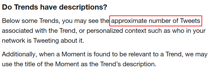
Check out this FAQ on Twitter trends.
How do we build one?
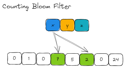
The structure of CountMinSketch is incredibly close to that of the Counting Bloom Filter. In a Counting Bloom Filter, we had one set of buckets with counters (m). Based on the output of all hash functions, the counters in this one bucket was incremented.
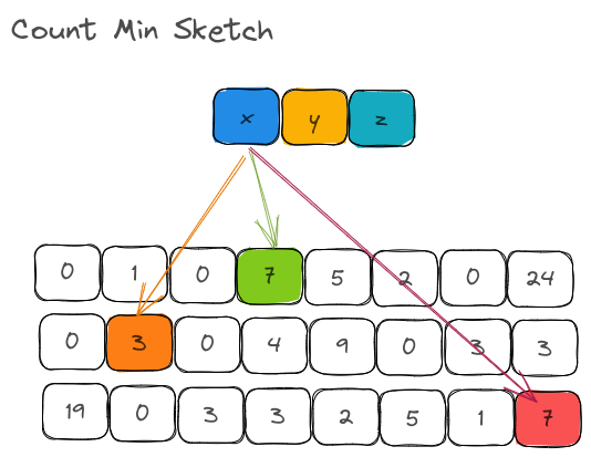
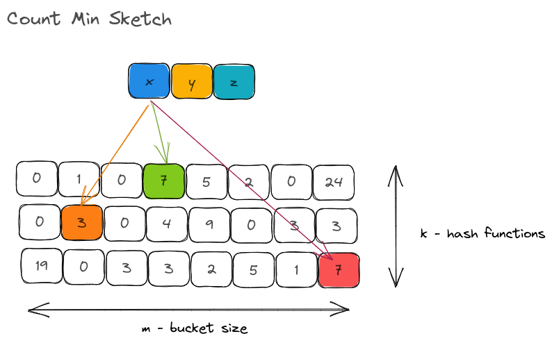
With CountMinSketch, we create one bucket of size m per hash function:
I believe I am breaking all the suspense here. This structure answers one big question that we had in mind:
Why does CountMinSketch better than Counting Bloom Filter for estimating frequency/counts?
By using m counters per hashing function instead of m counters for ALL hashing functions put together, we are able to significantly reduce the number of collisions that would happen on the bucket. Of course, the downside is that we now need space for k * m counters instead of 1 *m counters but the estimates are very close to the actual counts.
Properties
Before we implement the data structure, let us get the properties summarized:
- We saw that a CMS solves the "frequency" problem by enabling us to estimate frequencies of elements in streaming systems and/or in large datasets.
- It uses multiple hash functions and each hash function uses its hash output to increment counters in their own dedicated buckets, for keeping track of frequencies.
- They use very less memory in comparison to our traditional hashtable.
- You can only insert elements and get their estimated count. Deletion, updation, or iteration of values is not possible.
Implementation
1. Input parameters
There are two important parameters that CMS expects from the users - epsilon and delta. Hehe. I got you, didn't I? Let me elaborate it.
epsilon : Considering the estimated_count of an element is an approximation, you would want to control how closer to the actual count should the approximation be. The epsilon parameter is nothing but the maximum variance in the estimated count (or maximum allowable error rate). So, if you say the epsilon is 1%, and your estimated count is 1000, it means that the actual count could be between 990 and 1110. Now, why would someone not want the best possible estimate? The reason is that more accuracy comes at the price of more space (number of buckets).
delta : Since CMS is a probabilistic data structure, there could be false positives. In a Bloom Filter, the false positive rate of 1% means that approximately 1% of the time, the Bloom filter would say that an element is present in the set, while it was not. In order to minimize the false positive rate, in a bloom filter, we would typically increase the number of buckets and/or increase the number of hash functions.
In a CMS, a false positive rate of 1% would mean that 1% of the time, the count returned by CMS is incorrect - meaning 1% of the time the count is beyond the allowed error range specified by epsilon. Just like a Bloom Filter, a larger bucket and a higher number of hash functions are common approaches to reduce the false positive rate.
So, here's our implementation. For the purposes of simplicity, the counters are 32-bit unsigned integers but it is very common to see other variations.
2. Declaring the struct and instantiation
#[derive(Debug)]
pub struct CountMinSketch<K: Hash + Eq> {
    epsilon: f64,
    delta: f64,
    hasher: SipHasher24,
    counter: Vec<Vec<u32>>,
    m: usize,
    k: usize,
    len: usize,
    _p: PhantomData<K>,
}

impl<K: Hash + Eq> CountMinSketch<K> {
    pub fn new(max_variance_in_count: f64, fp_rate_of_count: f64) -> Result<Self> {
        let epsilon = max_variance_in_count;
        let delta = fp_rate_of_count;
        let m = optimal_m(delta);
        let k = optimal_k(fp_rate_of_count);
        let random_key = generate_random_key();
        let hasher = create_hasher_with_key(random_key);
        let counter = vec![vec![0_u32; m]; k];

        Ok(CountMinSketch {
            epsilon,
            delta,
            hasher,
            counter,
            m,
            k,
            len: 0,
            _p: PhantomData,
        })
    }
    ...
    ...
3. Hasher instantiation
We accept the epsilon and delta parameters and calculate the number of buckets (m) and the number of hash functions (k).
/// Generates a random 128-bit key used for hashing
fn generate_random_key() -> [u8; 16] {
    let mut seed = [0u8; 32];
    getrandom::getrandom(&mut seed).unwrap();
    seed[0..16].try_into().unwrap()
}

/// Creates a `SipHasher24` hasher with a given 128-bit key
fn create_hasher_with_key(key: [u8; 16]) -> SipHasher24 {
    SipHasher24::new_with_key(&key)
}
4. Number of buckets and hash functions
The formulas for arriving at optimal_m and optimal_k from epsilon and delta are :

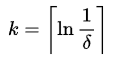
Their implementations being :
fn optimal_m(epsilon: f64) -> usize {
    (2.71828 / epsilon).ceil() as usize
}

fn optimal_k(delta: f64) -> usize {
    (1.0 / delta).ln().ceil() as usize
}
5. Building the APIs
Now that we have built the foundational functions, let's get into the API. There are just two functions to be implemented and both are very intuitive.
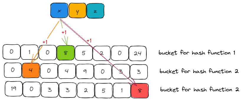
a. Insert
For every item that was inserted, we need to calculate k hashes. The methodology is the same as Counting Bloom Filter (section Hashers) where:
- we generate a 128-bit hash using
SipHasher - split them into two 64-bit hashes
- use Kirch and Mitzenmacher technique to create k-hash functions
- scoped down the hash to bucket indices of size
m - increment the counters corresponding to the bucket indices by 1.
impl<T: ?Sized + Hash + Debug> CountingBloomFilter<T> {
    pub fn insert(&mut self, key: &K) {
        let bucket_indices = self.get_bucket_indices(key, self.hasher);
        bucket_indices
            .iter()
            .enumerate()
            .for_each(|(ki, &bi)| self.counter[ki][bi] = self.counter[ki][bi].saturating_add(1));
        self.len += 1
    }


    /// Returns the bucket indices of k hash functions for an item
    fn get_bucket_indices(&self, item: &K, hasher: SipHasher24) -> Vec<usize> {
        let (hash1, hash2) = self.get_hash_pair(item, hasher);
        let mut bucket_indices = Vec::with_capacity(self.k);
        if self.k == 1 {
            let bit = hash1 % self.m as u64;
            bucket_indices.push(bit as usize);
            return bucket_indices;
        } else {
            for ki in 0..self.k as u64 {
                let hash = hash1.wrapping_add(ki.wrapping_mul(hash2));
                let bit = hash % self.m as u64;
                bucket_indices.push(bit as usize)
            }
        }

        bucket_indices
    }
b. Estimated count
The estimated count is calculated by hashing the item and looking into the counter values for each hash function. The minimal counter value is considered to be the estimated count.
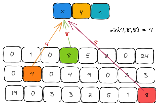
The reasoning behind choosing the minimum and not the maximum is that a counter could be incremented while inserting other elements due to hash collisions. Therefore, these counters overestimate the real frequency since the number of buckets is always much lesser than the number of items inserted into the sketch. Taking an average or a median is also not a fair estimate for items that have a lower frequency.
    pub fn estimated_count(&self, key: &K) -> u32 {
        let bucket_indices = self.get_bucket_indices(key, self.hasher);
        let mut estimated_count = u32::MAX;
        for (ki, &bi) in bucket_indices.iter().enumerate() {
            if self.counter[ki][bi] == 0 {
                return 0;
            } else {
                estimated_count = min(estimated_count, self.counter[ki][bi])
            }
        }
        estimated_count
    }
Test
    #[test]
    fn insert_and_check_several_items() -> Result<()> {
        let mut bf: CountMinSketch<&str> = CountMinSketch::new(0.2, 0.01)?;

        for _ in 0..1000000 {
            bf.insert(&"a1");
            bf.insert(&"a2");
            bf.insert(&"a3");
            bf.insert(&"a4");
            bf.insert(&"a5");
            bf.insert(&"a6");
            bf.insert(&"a7");
        }

        assert_eq!(bf.number_of_hashes(), 5);
        assert_eq!(bf.number_of_counters(), 272);
        assert_eq!(bf.estimated_count(&"a1"), 1000000);
        assert_eq!(bf.estimated_count(&"a2"), 1000000);
        assert_eq!(bf.estimated_count(&"b1"), 0);

        Ok(())
    }
Code
The complete code is here.